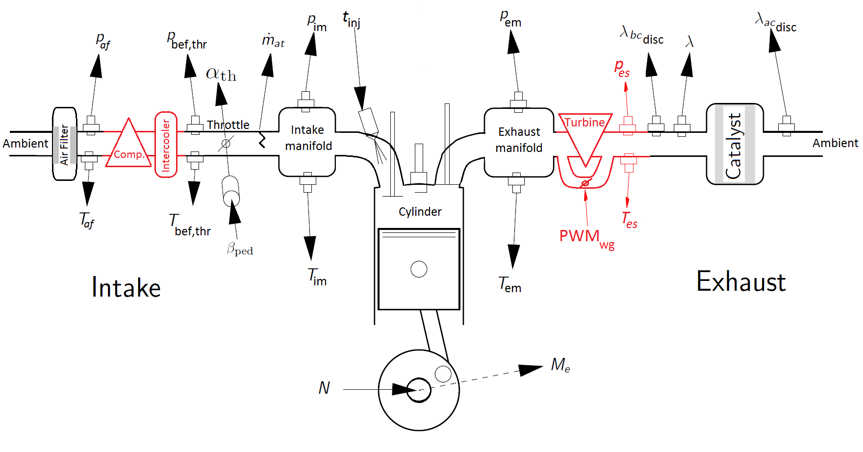
Figure 2.1: An overview of the air path with signals and components to be
modeled in project 1 (shown in black) and project 2 (shown in red+black)
Another major point of this template is that you will have everything at place. It will become easier for us to inform you and help you if you get stuck, but most of all it helps yourselves. What you write in Chapter 2 and what you do in preparatory tasks, is that you will build the rest of the work on. Just remember to bring your report and look at it when you are working on the project!
The template already contains a lot of text. Anything which is written in normal font is text that you can leave to remain. Text written in italics like this, you shall delete as it is only meant to be helpful to you while you write the report.
If you want to write in another word processing tool that is obviously fine, but the different sections and subsections must be well separated and easy to find.
You can choose to write your report in Swedish or English.
There are many constant parameters which are required in the models, it is your task to differentiate between the ones that need to be obtained from the measurements and those which relate to e.g. gas properties.
NOTE: In addition to the measurements required in Project 1, we also need to perform measurements for Project 2. These measurements are added with brief explanatory text in sections 2.8, and 2.9 below, and performed here to avoid duplicate measurement occasions. The star (⋆) before the section name indicates that these measurements are for Project 2. The projects 2 measurements are included in projects 1 report only the experiment plans (so you know what to measure and how), and thus not the implementation and validation of the models estimated from these measurements. Implementation and Validation for these components should instead be reported in project report for Project 2.
This project report deals primarily with a turbocharged engine. A mathematical model for the engine is to be developed and implemented, its model parameters identified from measured data, and the various models are validated. A controller in connected to the fuel injection system, which uses both feedforward and feedback from the discrete lambda sensor. Finally, the engine is coupled with a number of ready-made modules containing driver, clutch and driveline models. This is in order to perform simulations of the complete vehicle. A series of experiments are conducted with the aim to study the emission formation and consumption. The tool that is used for implementation is Matlab combined with Simulink.
Besides working on the engine model, the report addresses a series of studies, whose purpose is to illustrate how the energy stored in fuel is converted into a driving torque during the engine operating cycle, and the losses that may occur.
Project 1A.
In this chapter the engine is divided into a number of components, which are then
modeled separately. For each component specified input and output signals,
mathematical model which describes the behavior and the parameters are
determined. It is then described how the model parameters will be identified. An
overview of all input signals to the actuators and output signals from the sensors
which should be included in project 1 is shown in Figure 2.1 where the red
signals and components will be used in project 2 for a turbocharged engine.
Mathematical models are going to be used for the modeling of following engine sub components:
Because the simulations should be done with both warm and cold engine, it is also explored how long it takes for the catalyst to become warm. Sensors that measure air mass flow and pressure in the intake manifold are assumed to have negligible dynamics, while only the delays at lambda measurement are taken into account and exhaust gas mixing dynamics in the exhaust manifold are neglected. The control signals which are the inputs to the engine model are:
The control signals that are going to be mentioned in the experiment plans,
must be selected only among these. During measurements in the lab,
control signals are the ones which can be controlled from the control
room.
The entire engine model block in Simulink should produce the following output signals
For your convenience, a complete model description and experimental plan for the accelerator pedal, and most of model description for the throttle are already included in the report template. Use this as a template when you write model description and experimental plan for other components. You should have replaced every ???? in this template before submitting your report.
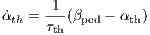
 | (2.1) |
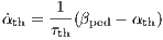
where βped and αth can changes continuously between 0 and 1.
 | (2.2) |
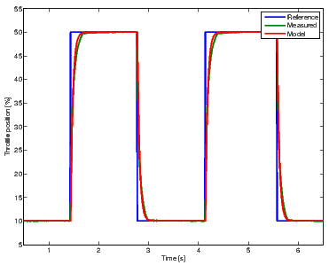
where t0 is the time point when the step happens. At time t = τth + t0 is
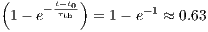 | (2.3) |
Therefore the time constant is determined as the time interval between the instance when the first change in the signal is observed until throttle angle reaches 63% of its final values.
The air mass flow past the throttle depends on throttle angle and ambient pressures and temperatures. In most of the engine operating points it is a significant pressure drop across the throttle which is well described by compressible flow models.
 |
which is also found in the textbook along with the expression for Ψ(Π). The only thing that is unknown is how the effective area Aeff depends on throttle plate angle αth. Here we use ...
Several models are proposed in the textbook, here a quadratic polynomial in αth is
recommended.
ṁat =  Aeff(αth)Ψ(Π), Aeff(αth)Ψ(Π), | Π | =  | (2.4) | |
| Aeff(αth) =???? | (2.5) | |||
Ψ =  , , | Πlim | = max | (2.6) |
Pressure dynamics in intake manifold. ????????????????????
????????????????????
In the cylinder model there is one sub-model for the generated torque, one sub-model
for the engine temperature and another one for the air/fuel ratio inside the cylinder
(λcyl).
tips: Equation 7.55 in the book is recommended for torque modeling, read chapter
7.9.[1,2,3] before doing this part. For friction modeling use the Heywood model on
page 191 but you have to find the model constants. For the temperature model, read
the project compendium.
Exhaust system is comprised of a model for exhaust manifold pressure and also the
light-off time for the catalyst.
Considering Figure 2.1, the fact that the Enginemap data is obtained from a
turbocharged engine and that a naturally aspirated engine is going to be modeled,
which one of Pem or Pes signals in the Enginemap should be used in this task?
Why?
tips: The output mass flow from the exhaust manifold can be modeled as an
incompressible turbulent restriction, see chapter 7.2 in the book.
????????????????????
models for continuous and discrete lambda sensors, before catalyst are required.
As part of the compressor model for Project 2, the outer wheel diameter of compressor impeller (dC2) is needed. This can most easily be measured by using calipers. In the same way, the turbine inlet diameter (dT1) should be measured with calipers.
Wastegate position of a turbocharged engine is normally controlled by the pressure on one side of a membrane. Pressure on other side of the membrane is normal ambient pressure. The pressure is controlled by using a mixing valve, where two sources with different pressure alternately are connected to the pressure chamber of the wastegate. This mixing valve is controlled by a PWM signal. An overview of the various components included in the wastegate controller on the turbocharged engine lab is shown in Figure 2.2.
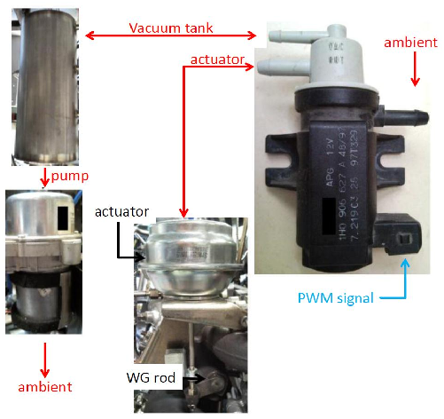
The PWM signal alternates between +5 V and ground, and the relative length difference between the +5 V level and ground-level controls the valve behavior. The frequency of the PWM signal is so high that an almost continuous signal is obtained (ie change between +5 V and ground occurs with the order of hundred Hz, because wastegate system frequency is significantly lower). The position of the wastegate arm can be measured in lab, and the PWM signal to the mixing valve can be controlled if wanted. A first order behavior, as for throttle angle, is assumed here. Model description and experiment plan for the wastegate will therefore largely follow the accelerator pedal.
Now that models are described and input-output-control signals are defined for all components, the block diagram of entire engine model can be illustrated as shown in Figure 2.3.
Project 1B.
The enginemap can be downloaded from:
www.fs.isy.liu.se/Edu/Courses/TSFS09/Projekt1/EngineTests/
This chapter outlines and discusses the results of projects 1B. The aim in projects 1B is to show how engine torque can be produced from chemically stored energy, and where losses can occur. Approach is described by presenting the utilized equations and the name of the used data file(s). The results of parameter estimations in models of different engine components are also reported and the models are validated against measurements.
This chapter will be submitted as the second submission, i.e. after the project 1B has been implemented. Attach the Matlab code.
Preparatory tasks need not be explained in the report, but be aware that they can provide valuable clues as you e.g. explain figures.
In this section, the models developed in previous chapter are compared against the measurement data.
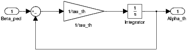
The accelerator pedal takes pedal position (βped) as input and provides throttle angle (αth) as output. The model is described by the equation:
 | (3.1) |
The model of the throttle determines the air mass flow rate into the intake manifold based on throttle angle. Model equation presented in Section 2.2, is repeated here
ṁat =  Aeff(αth)Ψ(Π), Aeff(αth)Ψ(Π), | Π | =  | |||||
| Aeff(αth) = ... | |||||||
Ψ = 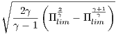 , , | Πlim | = max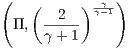 |
After validation of models, all estimated parameters in different sub models must be presented in this table. This makes it easier for us to correct your reports, and for you to reach and find different values during model implementation in Simulink.
All estimated parameters in the different engine sub models are summarized in table 3.1.
| Component | Parameter | Value |
| Accelerator pedal | τth | 0.??? [sec] |
| Throttle | . | ... |
| . | ... | |
| Intake manifold | . | ... |
| . | ... | |
| Fuel injector | . | ... |
| . | ... | |
| Cylinder | . | ... |
| . | ... | |
| . | ... | |
| Exhaust system | . | ... |
| . | ... | |
| Lambda sensor | . | ... |
Number of empty rows in front of each component is randomly selected and should not be inferred as number of parameters.
Project 1C.
This chapter presents how different models for sub components of the engine are
implemented in Simulink.
Project 1C, continued.
A fuel controller is connected to the engine fuel injection system. In this chapter, the
design of the controller, the way we went about it to determine the controller
parameters, and figures showing that we have succeeded are presented. A step in
accelerator position is implemented, and the plausibility of the results is
assessed.
Project 1C, continued.
This chapter first presents the results of a number of experiments specified in
the project compendium. The results are discussed and the plausibility is
assessed.
Include figures for: Continuous Lambda, Engine speed, Engine torque, Vehicle Speed VS drive cycle speed
Include figures for: Continuous Lambda, Engine speed, Engine torque, Vehicle Speed VS drive cycle speed
Project 1C, continued.